Framework

This page is the specification of the learning framework. The decision for the framework is of 2 October 2026. The Lean models in Verification/ are the source of truth for each formula on this page. The code must implement the Lean models.

Each item has one of three states.

State	Meaning
Exists	The code is in the repository and its tests pass
Specified, not built	The Lean model and this page give the rules. The production code is not in this release
Planned	The item is on the roadmap. This page gives no rules for it

The cited papers motivate the design choices. Results from other tasks are not measurements of ACRES.

Rule

The planner carries the horizon. The learned policy corrects the steering and the speed.

1. The exact planner and the mission automaton own the mission: the field order, the phases and the reference path.
2. Reinforcement learning never owns the mission. It adds a bounded residual to the pure-pursuit command for one leg.
3. A deterministic shield has the last word on each command. Training and deployment use the same shield.
4. Lean 4 supplies guarantees and training signals: the shield, the shaped reward, the automaton and the reward properties.

State of the Items

Item	State	Location
Planner: cost tables, option graph, exact dynamic programme	Exists; Lean model and proofs	planners/costs.py, options.py, solvers.py
Reference path: route graph, Dubins and Reeds–Shepp turns, loops	Exists	tasks/scouting/routes.py, reeds_shepp.py
Reference driver: pure pursuit and speed profile	Exists	tasks/scouting/reference_driver.py
Phase sequence by milestones	Exists	tasks/scouting/mission.py (EpisodeTracker)
Gear logic	Exists, proved	tasks/scouting/spec.py (GearManager)
Drive-by-wire command queue and watchdog	Exists, proved	Acres/Source/Acres/AcresCommandTiming.h, AcresUtvModel.cpp
Action limits of the command map	Exists, proved	tasks/scouting/spec.py (action_to_command)
Rewards v1 and bounded	Exists, proved in part	tasks/scouting/rewards.py
Flat PPO trainer and its tools	Exists	adapters/ppo/
Deployment program with the drivers reference and ppo	Exists	deploy/
Residual law	Specified, not built; Lean model and proofs	tasks/scouting/residual.py
Shield	Specified, not built; Lean model and proofs	tasks/scouting/shield.py
Mission automaton as a module	Specified, not built; Lean model and proofs	tasks/scouting/automaton.py
Residual reward with the shield term and the shaping term	Specified, not built; Lean model and proofs. The constants are in configs/scouting_v1.json (rewards_residual)	tasks/scouting/rewards.py
Plan checker	Specified, not built; Lean model and proofs
Residual-policy observation	Specified, not built	tasks/scouting/observations.py
Segment episodes	Specified, not built	adapters/ppo/curriculum.py, envs/scouting.py
Whole-mission evaluator	Specified, not built	eval/missions.py
Deployment driver residual with the gain \(\alpha\)	Specified, not built	deploy/drivers.py
Cost model of soil moisture, online slip estimate	Planned

All code paths are under Learning/acres_learn/ unless the table gives a different root. The Lean models are in Verification/AcresVerification/ (Shield/, Mission/, Shaping/, Reward/, Planner/). The golden vectors in Verification/Differential/golden/ are the test of the production code. Commit 58457c4 preserves an early draft of shield.py and automaton.py in Git history. The draft predates the Lean models and does not agree with them. The active code excludes that draft.

Decisions

These decisions are of 2 October 2026, after the Lean development.

Subject	Decision
Source of truth	The Lean models. This page and the code follow them
Shield penalty	0.5 for each step with an intervention, subtracted after the bounded map
Failure penalties of the residual variant	−1200 for each failure; −1500 for a collision (rewards_residual)
Shield rules	The rules of the Lean model. The first statement of the rules had errors (Findings)
Obstacle distance	Measured along the output curvature. Two calls: shield_curvature, then shield
Stage order in a control step	Driver, residual, launch hold, shield, gear logic, actuator clip. The shield is the last stage that can increase or change a command
Events	A failure has priority when two events occur in one control step. HOME_STOPPED is the completion test

Reasons

A flat policy is one network that drives the whole mission. The flat PPO runs reached 69 % on the GoTo phase and 0 of 64 on whole missions (Results). The following studies motivate this design; their tasks and measurements differ from ACRES.

• TADPO tested PPO, PPO with behaviour cloning, SAC and DAgger on sparse-waypoint off-road driving. All four scored 0 % (TADPO).
• PRM-RL reached 91.7 % success on three floorplan maps with dense roadmaps. The margin over pure AutoRL was 83.2 percentage points (PRM-RL).
• CaRL trains PPO with a route as input. On CARLA longest6 v2, its driving score is 64; PDM-Lite scores 73. PDM-Lite also uses scenario information that CaRL does not receive (CaRL).
• Lee et al. use Dijkstra for global routes and learned local control on kilometre-scale missions. Their training waypoints are 2 to 20 m apart (Lee et al.).

The table connects the observed failures to related work and proposed changes. Evaluation must test whether these changes help ACRES.

Failure of the Flat Runs	Published Counterpart	Remedy
The first update after a stage change moved the policy by a KL of 8.9	Destructive updates at a hand-over (PIRLNav)	No stages. A critic-only warm-up at the start
The policy forgot the garage exit	Forgetting in fine-tuning (Wołczyk et al.)	The garage exit is in each batch
A crash was cheaper than a bad continuation	Additive rewards and local minima (CaRL)	Bounded step reward. Failures never pay
The distance-to-go input left the range of the normaliser	Path-conditioned planner (Haro et al.)	Direction and log-distance encoding. No distance-to-go input
Phase joins failed (GoTo to Scout, Scout to Return)	A subtask level is necessary (pi0.5)	The automaton owns the phases

Layers

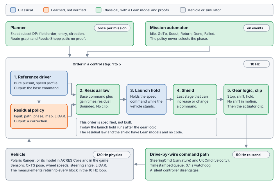
Layer	Component	Rate	Kind	State
Mission order	Exact dynamic programme over subsets of fields	One time for each mission	Classical, proved exact	Exists
Phases	Mission automaton	On events, tested at 10 Hz	Classical, proved	Specified, not built
Reference path	Route graph, turns, loops	One time for each mission	Classical	Exists
Base driver	Pure pursuit and speed profile	10 Hz	Classical	Exists
Residual	PPO actor	10 Hz	Learned, not verified	Specified, not built
Launch hold	spec.LaunchHold	10 Hz	Classical	Exists, before gear control
Shield	Action replacement	10 Hz	Classical, proved	Specified, not built
Gear logic	spec.GearManager	10 Hz	Classical, proved	Exists
Command path	Timestamped queue and watchdog	120 Hz physics; re-send at 50 Hz	Classical, proved	Exists

Order in a Control Step

State: specified, not built.

1. The base driver gives the base command.
2. The residual law adds the residual. It does not clip the command.
3. The launch hold can hold the speed command while the vehicle stands.
4. The shield gives the safe command.
5. The gear logic makes the stop, the GearCmd and the hold of a gear change.
6. The clip of spec.command_rows applies the actuator limits. It does not change the output of the shield (limited_shield).

The shield is the last stage that can increase or change a command. The gear logic can only replace the speed by 0. The current code puts launch hold before speed caps and gear logic. The production shield must go between launch hold and gear logic.

Interfaces

From	To	Data
Planner	Automaton, base driver	The plan: for each field its identifier, entry, direction, access point and exit point. The legs: for each phase a path with points 1 m apart. Each point has a ground class, a speed limit \(v_\text{max}\) and a direction of travel (+1 or −1)
Automaton	Residual policy, evaluator	The phase and the leg index
Vehicle	Base driver	The pose \((x, y, \psi)\) in the map frame and the forward speed
Base driver	Residual law, shield, residual policy	The base command \((\kappa_\text{PP}, v_\text{PP})\): a curvature in m⁻¹ (left is positive) and a signed speed in m/s
Residual policy	Residual law	\(a = (a_0, a_1)\)
Residual law	Shield	The proposed command \((\kappa, v)\), without a clip
Shield	Gear logic	The safe command, the flag intervened and the rule codes violated
Gear logic	Drive-by-wire	SteeringCmd in curvature mode, UlcCmd in velocity mode, GearCmd at standstill

The control step is \(\Delta t = 0.1\) s. The watchdog of the drive-by-wire disengages a subsystem 0.1 s after its last command.

Residual Law

State: specified, not built. Lean model: Shield/Residual.lean.

\[ \kappa = \kappa_\text{PP} + g \, a_0 \, \Delta\kappa, \qquad \Delta\kappa = 0.05 \text{ m}^{-1} \]

\[ v = v_\text{PP} + g \, a_1 \, \Delta v, \qquad \Delta v = \begin{cases} 0 & \text{if } v_\text{meas} \text{ or } v_\text{PP} \text{ is not finite} \\ 0 & \text{if } \lvert v_\text{meas} \rvert < 0.3 \text{ m/s} \\ \min(1.0 \text{ m/s},\; 0.3 \, \lvert v_\text{PP} \rvert) & \text{otherwise} \end{cases} \]

Symbol	Definition
\(g\)	The gain \(\alpha\) after the clamp to \([0, 1]\). A NaN gain gives \(g = 0\)
\(a_0, a_1\)	The policy output after the action clip of the task: a NaN becomes 0, then the clip to \([-1, 1]\)
\(v_\text{meas}\)	The measured forward speed

These rules are part of the law.

• If \(g\) is not above 0, the law returns the base command itself. It does not calculate base + 0 * x. Thus the bits of the base command pass. This includes a base speed of -0.0.
• The code calculates base + gain * a * delta from left to right. \(\lvert x \rvert\) is abs(x).
• The command of the law goes to the shield without a clip. The actuator clip is at the end of the command path.
• The code checks the configuration when it loads it. Each value must be finite. No range can be negative. The share of the base speed must be at most 0.5.
• Training uses \(\alpha = 1\).

The law has these properties. Each one has a Lean proof.

Property	Statement	Theorems
Identity at zero gain	\(\alpha \le 0 \Rightarrow (\kappa, v) = (\kappa_\text{PP}, v_\text{PP})\), bit for bit	compose_zero_gain, compose_zero_gain_float
Curvature bound	\(\lvert \kappa - \kappa_\text{PP} \rvert \le 0.05 \, g\) m⁻¹	compose_deviation, residualCommand_deviation
Speed bound	\(\lvert v - v_\text{PP} \rvert \le g \min(1.0,\; 0.3 \lvert v_\text{PP} \rvert)\) m/s	residualCommand_deviation
Sign	\(v\) has the sign of \(v_\text{PP}\). If \(v_\text{PP} = 0\) then \(v = 0\)	residualCommand_sign
Standstill	While \(\lvert v_\text{meas} \rvert < 0.3\) m/s, \(v = v_\text{PP}\) as a number	residualCommand_standstill
Monotone	The deviation from the base command does not decrease when the gain increases	deviation_mono_gain

The sign property has two effects. The residual cannot ask for a gear change. The residual cannot move the vehicle when the base command is a stop.

The speed after the shield is not monotone in the gain. A larger gain can make the arc tighter and decrease the corner limit (shielded_speed_not_monotone_in_gain).

The law is the form of RLPP, which used a gain of 0.55 on a real 1/10-scale car (RLPP). The evidence on full-size vehicles is thin. One study found that a residual on a model-predictive base can make the performance worse on hardware (reset-free RL). The gain \(\alpha = 0\) is the answer to that risk.

Observation

State: the proprioception, map crop and LiDAR groups exist. The path group below and the critic group are specified, not built. They have no Lean model.

Group	Size	Content	Receiver
Proprioception	13	Speed, yaw rate, lateral acceleration, steering wheel angle, pitch, roll, four wheel speeds, gear, previous command (2 values)	Actor and critic
Path	136	16 waypoints with 8 values each, then 8 scalar values	Actor and critic
Map crop	4 × 64 × 64	Crop, edge band, lane or verge, obstacle. 32 m square at 0.5 m. No soil water	Actor and critic
LiDAR	360	Planar ranges, 1° apart, 30 m	Actor and critic
Critic	2	Remaining reference time; end-of-mission flag	Critic only, training only

The previous command is the final command of the last control step, after the shield, as a normalised action.

Path Encoding

The path group uses the encoding polar_log. Waypoint \(i\) (\(i = 1 \ldots 16\)) is on the mission path at the arc length \(s^* + 2i\) m. \(s^*\) is the furthest arc length that the vehicle reached on the current leg. The waypoints continue into the next leg past the end of the current leg. \((x_i, y_i)\) is the waypoint in the body frame, with x forward and y left. \(d_i = \sqrt{x_i^2 + y_i^2}\).

Value	Definition
1, 2	Direction: \(x_i / d_i\) and \(y_i / d_i\). For \(d_i = 0\) the direction is (1, 0)
3	\(\log(1 + d_i)\), with \(d_i\) in metres
4, 5, 6	Ground class of the waypoint, one-hot: lane, verge, edge band
7	Speed limit \(v_\text{max}\) of the waypoint, m/s
8	Direction of travel: +1 forwards, −1 backwards

The 8 scalar values are:

Value	Definition
1	Cross-track error \(e\) in metres. Positive: the vehicle is left of the path
2	Heading error in radians: vehicle heading minus direction of travel of the path, in \([-\pi, \pi)\)
3, 4	Base command: \(\kappa_\text{PP}\) (m⁻¹) and \(v_\text{PP}\) (m/s)
5	Speed cap \(c\) of the path (m/s)
6, 7, 8	Automaton phase, one-hot: GoTo, Scout, Return

The phase input has one bit set in a driving state and no bit set in the other states (phaseOneHot_spec).

The actor gets no distance-to-go and no time-left value. This is the encoding of a path-conditioned planner (Haro et al.). In the flat runs, the distance-to-go input reached 10 standard deviations outside the training range on long routes.

Critic Group

Value	Definition
1	\(N_\text{ref}(s^*) \, \Delta t / 60\): the remaining reference time of the episode path in minutes, from the progress point \(s^*\) that the potential uses
2	1 if the end of the episode path is the end of the mission, else 0

The shaped value of a state is \(V - \Phi(s^*)\) (value_shape). The potential \(\Phi\) is a function of \(N_\text{ref}(s^*)\). Thus the critic must see \(N_\text{ref}\). The exported policy has no critic. Thus the vehicle does not need these values.

Segment Episodes

State: specified, not built. The episodes have no Lean model. The truncation rule has one (Shaping Term).

A training episode is one segment. There is one stage and no curriculum.

Property	Rule
Missions	The single-field missions of the 43 training fields. Each mission uses its frozen optimal plan
Phase shares	Garage exit 15 %, GoTo 30 %, Scout 35 %, Return 20 %
Garage exit	The vehicle starts at H, at rest. The segment is the start of the GoTo leg
Other starts	A point of the leg where the travel is forwards and the plan box is 0.5 m clear of obstacles
Start state	On the path at the speed of the reference profile. Lateral offset uniform in ±0.5 m. Heading error uniform in ±5°
Length	Uniform from 120 to 300 m. The end of the leg ends the segment earlier
Base driver	It follows the full remaining mission path. It does not brake for the end of the segment
Path input	It continues past the end of the segment along the mission path
End of the segment	Reached when \(s^*\) is within 2 m of the end. This is a truncation
Time limit	1.5 times the reference time of the segment plus 10 s. This is a truncation
Terminations	Collision, stuck, deep in crop, left the map, lost (10 m outside the corridor), stopped at H
Soil water	Uniform from 0.5 to 1.3 for each episode
Drive-by-wire parameters	Drawn at half of their fitted spread for each episode
Sensor noise	Full scale (Training)

The reasons are:

• A segment has no stage change. Thus no update comes after a change of the task.
• The garage exit is in each batch. Thus the policy cannot forget it.
• A truncation at the end of the segment keeps the unshaped value independent of the segment length. The shaped value has the additional term \(0.55 \, N_\text{ref}(s^*)\). The critic gets \(N_\text{ref}\) as an input.
• The end of a segment has no milestone bonus. Thus no reward depends on a point that the actor cannot see.

Validation. The validation drives the whole single-field missions of the 6 validation fields. The actions are the means of the policy. The shaping term is off.

Reward

State: the terms of v1 and the bounded map exist. The residual variant is specified, not built. Lean model: Reward/Residual.lean, Shaping/Model.lean. The constants are in configs/scouting_v1.json (rewards_residual).

The residual trains on the variant env.rewards = "residual" (residualReward_eq).

\[ r'_t = B(d_t) - w_s \, 1_\text{intervention} + e_t + F_t \]

Constant	Value	Configuration Key
Knee and floor of the bounded map	−2, −5	rewards_bounded.step_knee, step_floor
Shield penalty \(w_s\)	0.5	rewards_residual.shield_per_step
Shaping weight \(c_\Phi\)	0.55 for each reference control step	rewards_residual.shaping_cost_per_step
Discount \(\gamma\)	0.995	rewards.gamma; must be equal to ppo.gamma
Stuck, deep in crop, left the map, lost, stalled	−1200 each	rewards_residual.stuck, deep_in_crop, left_map, lost, stalled
Collision	−1500	rewards_residual.collision

The section rewards_bounded (−1000, −1250) does not change. The earlier runs use it.

Dense Sum

\[ d_t = r^\text{prog}_t + r^\text{cover}_t + r^\text{time}_t + r^\text{energy}_t + r^\text{crop}_t + r^\text{presence}_t + r^\text{track}_t + r^\text{smooth}_t + r^\text{safe}_t + r^\text{gear}_t \]

\(d_t\) is the dense sum of the bounded variant. It has no shield term.

Term	Formula	Constants
Progress	\(w_p \, (s^*_t - s^*_{t-1})\)	\(w_p = 2.5\) m⁻¹
Coverage	\(b_c\) for each newly covered checkpoint in a Scout phase; 0 on a step in crop	\(b_c = 0.5\)
Time	\(-c_t\)	\(c_t = 0.25\)
Energy	\(-w_E \, (\Delta E_\text{fuel} + \lambda_g \Delta E_\text{ground}) / E_\text{ref}\)	\(w_E = 0.3\), \(\lambda_g = 1\), \(E_\text{ref} = 2689.8\) J
Crop	\(-(w_c \, \Delta A^\text{crop} + w_{ce} \, \Delta A^\text{edge}) / A_\text{ref}\)	\(w_c = 5\), \(w_{ce} = 0.2\), \(A_\text{ref} = 0.636\) m²
Crop presence	\(-P\) if a part of the shrunk plan box is on crop outside the edge band	\(P = 1\), shrink 0.5 m
Tracking	\(-w_e \max(0, \lvert e \rvert - h)^2\), \(h = \max(0, h_\text{side} - 0.8)\)	\(w_e = 0.5\) m⁻²
Smoothness	\(-w_a \lVert a_t - a_{t-1} \rVert^2\) on the final commands as normalised actions	\(w_a = 0.05\)
Safety	\(-w_o \lvert v \rvert \max(0, 1 - (d_\text{min} - 2)/8)\)	\(w_o = 0.2\) s/m
Gear	\(-w_g\) for each GearCmd	\(w_g = 0.5\)

Field Scouting Task gives the reasons for the weights.

The code must add the terms in this order. The golden vectors compare bits. rewards.bound(dense) is the correction \(B(d) - d\). Thus the sum of the dense terms and of bound is \(B(d)\).

dense  = sum(progress, coverage, time, energy, crop, crop_presence, tracking, smoothness, safety, gear)
bound  = rewards.bound(dense)
shield = -shield_per_step if the shield intervened, else 0.0
reward = sum(progress, coverage, time, energy, crop, crop_presence, tracking, smoothness, safety, gear,
             events, bound, shield, shaping)

Bounded Map

\[ B(d) = \begin{cases} d & \text{if } d \ge -2 \\ -2 - \dfrac{3x}{x + 3}, \quad x = -2 - d & \text{if } d < -2 \end{cases} \]

\(B(d) > -5\) for each \(d\). \(B\) is strictly increasing. The reward subtracts the shield term after the map. Thus a step that is not a failure earns more than −5.5 before its events and its shaping term (penaltyOutside_gt).

These statements are for exact numbers. In doubles, \(B\) keeps the order of two steps only up to rounding (\(4 \times 10^{-15}\), bounded_not_monotone). In doubles, \(B\) reaches −5 at \(d \approx -3 \times 10^8\). It is exactly −5 at \(d = -10^9\) (bounded_reaches_floor). The first value needs a position 25 km outside the corridor. The tile is 1.5 km wide.

Shield Term

A step in which the shield changed the command pays \(-w_s = -0.5\). The reward subtracts the term after the bounded map. Thus it has its full value in each state. Inside the map it is worth only 0.005 at \(d = -29\) (intervention_cost_small).

Events

Event	Value	Condition
Stopped at H	+50	The mission is complete. In a segment episode: the vehicle is stopped at H at the end of the Return leg
Entry reached, field scouted	+10, +50	Whole-mission episodes only. A segment episode does not pay them
Collision	−1500	Termination
Stuck, deep in crop, left the map, lost, stalled	−1200 each	Termination

The failure values satisfy two inequalities (spec_failure_inequalities).

1. Like for like. \(F \le (-5 - w_s) / (1 - \gamma) = -1100\). The comparison needs a continuation value of at least \(F - 5.5\) (spec_failure_event_never_pays). It does not cover a later, more severe failure. The value −1200 gives a margin of 100 against the bound −1100.
2. Against each continuation without a failure. \(D_\text{max} + E_\text{hi} + F < -1100\). \(D_\text{max} = 2.5 \times 14 + 0.5 \times 4 - 0.25 = 36.75\) is the largest dense reward of one step (dense_le_of_limits). \(E_\text{hi} = 50\) is the largest milestone on a step with a failure. Then \(36.75 + 50 - 1200 = -1113.25\). The margin is 13.25 (spec_failure_cross_step). The value −1150 does not satisfy the inequality.

The collision is the worst failure: \(-1500 \le -1200\).

The second inequality uses limits of one control step that come from the code. They are hypotheses of the proof (StepLimits, specMilestoneMax). They are not theorems.

Hypothesis	Value	Source in the Code
Progress of one control step	\(\Delta s^* \le 14\) m	mission._project searches 12 m ahead of \(s^*\) and takes the path segment after the first point past that distance
New checkpoints of one control step	At most 4	A coverage-disc check on the current map; a runtime count guard for the residual variant
Milestones on a step with a failure	At most one, of at most 50	entry_reached 10 or field_scouted 50. The code pays home_stopped only on a success

The runtime guard rejects progress above 14 m. Nominal path spacing does not establish this limit at a path join. Checkpoint spacing of 10 m and a coverage radius of 8 m do not establish the count limit on every possible outline. The map check tests the current geometry. A new map must pass this check.

If the code changes one of these limits, do the calculation of the second inequality again.

PPO reward units. The residual variant must use ppo.gamma=0.995, normalize_rewards=false and reward_clip=null. The trainer passes raw rewards to the value targets. It applies no running scale or reward clip.

The cast to float32 still introduces rounding; the exact-number proofs do not cover that rounding. The configuration validator keeps residual training disabled until the production framework exists. The historical flat PPO baselines retain their original reward processing.

A failure on a step with a positive dense reward can be worth more than a continuation at the floor. The Lean counterexample for the bounded variant is failure_pays_on_a_good_step. This is the reason for the second inequality.

Shaping Term

\[ F_t = \gamma \, \Phi(s^*_{t+1}) - \Phi(s^*_t), \qquad \Phi(s^*) = -c_\Phi \, N_\text{ref}(s^*) \]

The table \(N_\text{ref}\). Each episode has a table with one value for each point of the episode path.

Item	Definition
Segment time	The time of the reference speed profile for the path segment between two points. It is a term of deploy.mission.path_time_s: \(\Delta s\) divided by the mean speed of the segment (at least 0.3 m/s)
Value at the last point	0
Value at point \(i\)	The sum of the segment times after \(i\), divided by the control step. The sum starts at the end of the path
\(N_\text{ref}(s^*)\)	numpy.interp(s*, arcs, N): linear between the points, the total before the first point, 0 at and after the last point
Rounding	\(N_\text{ref}\) is a real number. The code does not round it
Condition	The arc lengths must not decrease

The table is well formed, and its total is the reference time of the episode in control steps (costToGoOfSteps_wellFormed, remaining_isCostToGo). \(-0.55 \, N_\text{total} \le \Phi \le 0\) (spec_potential_bounds).

The state of the potential. The potential uses only the reference plan and the progress \(s^*\). It is a function of the augmented state: the simulator state, \(s^*\) and the table of the episode. It is 0 in a terminal state. It is not a function of the vehicle position (no_potential_of_position, shapingStep_eq_aug).

Case	Rule
Normal step	\(F_t = \gamma \Phi(s^*_{t+1}) - \Phi(s^*_t)\)
Termination (failure, or stop at H)	\(\Phi(s_{t+1}) = 0\). Thus \(F_t = -\Phi(s^*_t)\)
Truncation (end of the segment, time limit)	\(F_t = \gamma \Phi(s^*_{t+1}) - \Phi(s^*_t)\) with the real next state. PPO bootstraps with the critic of the shaped problem
End of the episode path	At and after the last point of the path, \(N_\text{ref} = 0\) and \(\Phi = 0\)
End of a segment	The vehicle reaches the end within 2 m of the last point. There \(\Phi = -0.55 \, N_\text{ref}(s^*_T)\), which is not 0. The truncation rule applies
Validation and evaluation	\(F_t = 0\). The reports give the unshaped return

Truncation. The exact value of the shaped critic is \(V(s_T) - \Phi(s_T) = V(s_T) + 0.55 \, N_\text{ref}(s^*_T)\). Then the shaped return is the unshaped bootstrapped return minus \(\Phi(s_0)\) (shaped_boot_return, spec_truncation).

An error \(\varepsilon\) of the critic changes the shaped return by \(\gamma^T \varepsilon\) (shaped_boot_return_critic_error). Do not set \(\Phi(s_T) = 0\) at a truncation. That convention can reverse the order of two trajectories (terminal_convention_at_truncation_reverses). A truncation without a bootstrap can reverse it too (no_bootstrap_reverses).

Invariance. With these rules the shaped return of an episode that terminates is the unshaped return minus \(\Phi(s_0)\) (shaped_return_terminal). For a truncated episode with the shaped bootstrap value the same is true. The difference does not depend on the policy.

The shaped process and the unshaped process have the same optimal policies, the same greedy actions and the same advantages (optQ_shape, isOptimal_shape, advantage_shape). They also have the same order of each two policies (objective_shape_le_iff). This is the result of Ng, Harada and Russell (1999). The Lean proof is for a finite process with stationary policies (Shaping/Mdp.lean).

Steps of a stop and of a failure. The shaping term adds \((1 - \gamma) \, c_\Phi \, N_\text{ref} = 0.00275 \, N_\text{ref}\) to a step without progress. A driving step from the same progress point has the same term. The shaping adds \(\gamma \, c_\Phi \, \Delta N_\text{ref}\) more to the driving step (spec_shaped_step_difference). At a failure, the step carries \(-1200 + 0.55 \, N_\text{ref}\) (spec_failure_step_shaped). The order of the returns (failure < stop < lane) is the same with and without the shaping term (spec_attractor_order).

Bound. \(\lvert r' \rvert \le \max(1505.5,\; D_\text{max} + e_\text{hi} + 0.55 \, N_\text{total})\) (spec_reward_bound).

Shield

State: specified, not built. Lean model: Shield/Shield.lean.

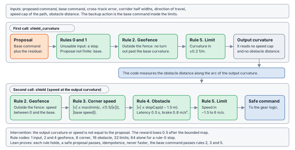
The shield is a deterministic function without state. Training, evaluation and deployment call the same function.

Parameters

Parameter	Symbol	Value
Curvature limit	\(\kappa_\text{max}\)	0.2 m⁻¹
Speed limits	\(v_\text{min}, v_\text{max}\)	−1.5 m/s, 6 m/s
Vehicle margin		0.8 m
Geofence margin		0.3 m
Lateral acceleration limit	\(a_\text{lat}\)	1.5 m/s²
Obstacle margin	\(d_m\)	1.5 m
Latency of a stop	\(\tau\)	0.5 s
Brake deceleration	\(a_b\)	0.8 m/s²

The code checks the parameters when it loads them (ShieldParams.wellFormed). Each value must be finite. \(v_\text{min} \le 0 \le v_\text{max}\). \(a_\text{lat}\) and \(a_b\) must be above 0. The other values must not be negative.

Inputs

Input	Definition
\((\kappa, v)\)	The proposed command
\((\kappa_\text{PP}, v_\text{PP})\)	The base command. It is the backup action
\(e\)	The signed cross-track error. Positive: the vehicle is left of the path, in the direction of travel
\(h_\text{left}, h_\text{right}\)	The corridor half widths at the projection: the metres of lane and verge on each side of the path. On an edge-band point the edge band counts too. The maximum is 8 m
direction	The direction of travel of the path at the projection: +1 forwards, −1 backwards
\(c\)	The speed cap of the path at the point where the base driver reads its speed
\(d_\text{obs}\)	The free distance from the vehicle to the nearest LiDAR return in the swept corridor of the output curvature. \(+\infty\) if there is no return within 30 m

\(e\), \(h_\text{left}\), \(h_\text{right}\) and direction must come from one projection onto one path segment. The sign of the base speed is not sufficient for the direction. Near a change of direction, the projection can be on a different stretch than the base driver.

The shield uses the base command inside the actuator limits.

\[ \kappa_b = \operatorname{clamp}(\kappa_\text{PP}, -0.2, 0.2), \qquad v_b = \operatorname{clamp}(v_\text{PP}, -1.5, 6) \]

Call Sequence

1. The code calls shield_curvature. The result is the output curvature \(\kappa_\text{out}\). This call reads neither \(c\) nor \(d_\text{obs}\) (shieldCurvature_independent).
2. The code measures \(d_\text{obs}\) along the arc of \(\kappa_\text{out}\). The corridor is behind the vehicle when the proposed speed is negative. If the proposed speed is not finite, the sign of \(v_b\) decides.
3. The code calls shield. Its output curvature is the result of step 1 (shield_curvature_eq).

Rules

Each rule is an interval for the curvature or for the speed. The shield clamps the value into each interval.

Rule 0. Unusable inputs give a stop. If \(\kappa_\text{PP}\), \(v_\text{PP}\), \(e\), \(h_\text{left}\), \(h_\text{right}\), direction or \(c\) is not finite, the output is \(v = 0\) and \(\kappa = \kappa_b\). If \(\kappa_\text{PP}\) is not finite, \(\kappa = 0\). If \(d_\text{obs}\) is NaN or \(-\infty\), the output is \(v = 0\) with the output curvature of rules 1, 2 and 5. The rule code is 64.

Rule 1. Proposal that is not finite. A proposed \(\kappa\) that is NaN or infinite becomes \(\kappa_b\). A proposed \(v\) that is NaN or infinite becomes \(v_b\).

Rule 2. Geofence. The fence is inside the corridor edge by the vehicle margin and the geofence margin. The code calculates (h - 0.8) - 0.3, not h - 1.1. The two results are different doubles for \(h = 3\) m (fence_order).

\[ f_\text{left} = \max(0,\; h_\text{left} - 0.8 - 0.3), \qquad f_\text{right} = \max(0,\; h_\text{right} - 0.8 - 0.3) \]

\[ \text{out}_\text{left} = (e > f_\text{left}), \qquad \text{out}_\text{right} = (-e > f_\text{right}) \]

The curvature rule depends on the direction of travel.

Stretch	Outside on the Left	Outside on the Right
Forward (direction \(\ge 0\))	\(\kappa \le \kappa_b\)	\(\kappa \ge \kappa_b\)
Backward (direction \(< 0\))	\(\kappa \ge \kappa_b\)	\(\kappa \le \kappa_b\)

In reverse, the left of the path is the right of the vehicle (arc_lateral_sign). The rule assumes that the heading of the vehicle is within 90° of the stretch (forwards) or of its reverse (backwards). The shield has no heading input.

Outside the fence on a side, the speed is between 0 and \(v_b\):

\[ \min(v_b, 0) \le v \le \max(v_b, 0) \quad \text{if } \text{out}_\text{left} \text{ or } \text{out}_\text{right} \]

Outside the fence, a driver can only steer back relative to pure pursuit. It cannot add speed. A proposal against the direction of the base command becomes 0. The backup action is the pure-pursuit command.

Rule 3. Corner speed. The rule reads the output curvature \(\kappa_\text{out}\).

\[ \lvert v \rvert \le \max\Bigl(\min\bigl(c,\; \sqrt{a_\text{lat} / \lvert \kappa_\text{out} \rvert}\bigr),\; \lvert v_b \rvert\Bigr) \]

For \(\kappa_\text{out} = 0\) the cap is \(\max(c, \lvert v_b \rvert)\). The residual cannot add speed on an arc whose corner limit is lower. The base command passes.

The path cap \(c\) is the braking envelope of the path limit:

\[ c_i = \min_{j \ge i} \sqrt{v_{\text{max},j}^2 + 2 \, a_c \, (s_j - s_i)}, \qquad a_c = 1.5 \text{ m/s}^2 \]

\(v_{\text{max},j}\) is the path limit of point \(j\): the minimum of the class limit and the corner limit.

Limit	Value
Class limit	5 m/s on lane and verge; 3 m/s on the edge band
Corner limit	\(\sqrt{1.5 / \lvert \kappa_\text{path} \rvert}\): a lateral acceleration of 1.5 m/s²
Backward limit	1.5 m/s on a backward stretch

The shield reads \(c\) at the arc length \(s + 0.5 \text{ s} \cdot \lvert v_\text{meas} \rvert\). The base driver reads its speed profile at the same point. A vehicle within the cap that brakes at \(a_c\) arrives at each later point at or below the limit of that point (envelope_le, envelope_reaches).

Rule 4. Obstacle stop distance. The stop distance of a speed is \(\text{stop}(v) = v \, \tau + v^2 / (2 a_b)\).

\[ \lvert v \rvert \le \text{stopCap}(d_\text{obs} - d_m) \]

\[ \text{stopCap}(x) = \begin{cases} \dfrac{2x}{\tau + \sqrt{\tau^2 + 2x / a_b}} & \text{if } x > 0 \text{ and the denominator is above 0} \\ 0 & \text{otherwise} \end{cases} \]

\(\text{stopCap}(x)\) is the largest speed with \(\text{stop}(v) \le x\) (le_stopCap_iff). The rule has no interval when \(d_\text{obs} = +\infty\). This is safe: \(d_m + \text{stop}(6 \text{ m/s}) = 27 \text{ m} \le 30\) m (no_return_is_safe). A shorter reach of the scan or a higher speed limit needs the reach as the distance.

Rule 5. Actuator limits.

\[ -0.2 \le \kappa \le 0.2 \text{ m}^{-1}, \qquad -1.5 \le v \le 6 \text{ m/s} \]

Order of the Rules

1. Rule 0 and rule 1.
2. The curvature: the geofence interval, then the actuator interval. The result is \(\kappa_\text{out}\).
3. The speed at \(\kappa_\text{out}\): the geofence interval, the corner interval, the obstacle interval, the actuator interval.

Each curvature interval holds \(\kappa_b\). Each speed interval holds 0. Thus the rules never contradict each other (stop_satisfies). The order of the rules of one channel does not change the output (shield_speed_order_free, shield_curvature_order_free). The one order that matters is between the channels: the corner rule must read the output curvature (corner_before_curvature_counterexample).

Swept Corridor

The LiDAR scan has 360 beams. Its origin is 2.5 m ahead of the rear axle. The rear axle follows the arc of the output curvature \(\kappa_\text{out}\), with the radius \(R = 1 / \kappa_\text{out}\). This geometry has no Lean model.

Case	Condition for a Return at \((x, y)\) in the Body Frame
\(\lvert \kappa_\text{out} \rvert < 10^{-4}\) m⁻¹	\(\lvert y \rvert \le w\)
Otherwise	\(\lvert R \rvert - w \le \rho \le \sqrt{(\lvert R \rvert + w)^2 + 3.42^2}\), with \(\rho\) the distance from the centre of the arc

The half width is \(w = 1.1\) m: 0.8 m of vehicle and 0.3 m of margin. The front of the plan box is 3.42 m ahead of the rear axle. \(d_\text{obs}\) is the distance along the arc minus 3.42 m. For a backward command, the corridor is behind the vehicle and the offset is 0.5 m.

Intervention and Rule Codes

intervened = not (k_out == k_in and v_out == v_in), with the IEEE 754 comparison of doubles (shield_intervened_eq). A proposal with a NaN is always an intervention. -0.0 and 0.0 are equal. This is the step that the shield term of the reward counts.

violated is the sum of the codes of the rules that the proposal breaks.

Code	Rule
1	A proposed value is not finite
2	Geofence, curvature
4	Geofence, speed
8	Corner speed, at the output curvature
16	Obstacle stop distance
32	Actuator limits
64 (alone)	Rule 0: unusable inputs, the output is a stop

For usable inputs, intervened is true if and only if violated is not 0 (shield_intervened_iff_violated). With code 64, intervened is false when the proposal is already the stop.

Properties

Each property has a Lean proof over the real numbers, for well-formed parameters.

Property	Statement	Theorems
Limits	For each input, the output is inside the actuator limits	shield_actuator
Rules hold	The output satisfies each enabled rule	shield_satisfies
No contradiction	For each input, the stop \((\kappa_b, 0)\) satisfies each rule	stop_satisfies
Least restriction	A proposal that satisfies each rule is the output	shield_least_restrictive
Idempotence	The shield applied to its own output gives the same output, without an intervention	shield_idempotent
Base command	The base command passes each rule but the obstacle rule. The output for the base command is \((\kappa_b, \operatorname{clamp}(v_b, \pm\text{stopCap}))\)	shield_base, shield_base_fixed
Never faster	For a finite proposal, the output speed is between 0 and the proposed speed	shield_speed_between, shield_abs_speed_le
Stop distance	The output speed is 0, or \(d_m + \text{stop}(\lvert v \rvert) \le d_\text{obs}\)	shield_stop_distance, shield_obstacle
Largest speed	The obstacle rule passes each speed that can stop in the distance	obstacle_cap_greatest
Lateral acceleration	\(v^2 \lvert \kappa \rvert \le \max\bigl(1.5,\; v_b^2 (\lvert \kappa_b \rvert + \lvert \kappa - \kappa_b \rvert)\bigr)\)	shield_lateral_bound

With \(\alpha = 0\) and usable inputs, the shield acts only when an obstacle is inside the stop distance.

In doubles, the test of the stop distance must compare the speed with \(\text{stopCap}\). A test of \(\text{stop}(\lvert v \rvert) \le d_\text{obs}\) in doubles needs a tolerance of \(10^{-12}\) m (stopCap_rounding).

The shield is part of the environment, not part of the policy. A projection inside the policy causes action aliasing in the gradients (Markgraf et al.). Action replacement with a penalty was the best shield in a benchmark (Krasowski et al.).

Mission Automaton

State: the tracker mission.EpisodeTracker implements these transitions today. The separate module is specified, not built. Lean model: Mission/Automaton.lean.

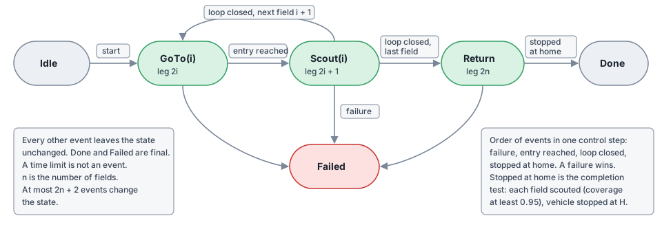
A mission has \(n\) fields. The state is a phase and a field index \(i\).

State	Meaning	Leg Index	Rank
IDLE	The mission has not started	0	\(2n + 2\)
GOTO(i)	The vehicle drives to the entry of field \(i\), \(0 \le i < n\)	\(2i\)	\(2(n - i) + 1\)
SCOUT(i)	The vehicle drives the loop of field \(i\)	\(2i + 1\)	\(2(n - i)\)
RETURN	The vehicle drives to H	\(2n\)	1
DONE	The mission is complete	\(2n + 1\)	0
FAILED	A failure ended the mission	\(2n + 1\)	0

In the code, \(n - i\) is max(n - i, 0). Only states with \(i < n\) occur in a mission.

State	Event	Next State
IDLE	START	GOTO(0) if \(n > 0\), else RETURN
GOTO(i)	ENTRY_REACHED	SCOUT(i)
SCOUT(i)	LOOP_CLOSED	GOTO(i+1) if \(i + 1 < n\), else RETURN
RETURN	HOME_STOPPED	DONE
GOTO(i), SCOUT(i), RETURN	FAILURE	FAILED
All states	Each other event	The same state

These rules apply to the events.

• DONE and FAILED are final.
• The time limit is not an event. An episode that runs out of time ends by truncation in its phase.
• Order of events. When more than one event occurs in a control step, the code gives them to the automaton in this order: FAILURE, ENTRY_REACHED, LOOP_CLOSED, HOME_STOPPED. Thus a failure has priority.
• LOOP_CLOSED is true when the vehicle is again at the entry where it joined the loop.
• HOME_STOPPED is the completion test of the task: each requested field is scouted (coverage at least 0.95), and the vehicle is stopped at H. This is necessary in each episode type that uses DONE as mission success.
• The automaton does not know the coverage. DONE means that each loop was closed and that HOME_STOPPED occurred.

Properties

Property	Statement	Theorems
Deterministic and total	Each state and each event have one next state	trans_deterministic, trans_total, trans_iff_step
Progress	Each event that changes the state, other than FAILURE, decreases the rank by 1. A FAILURE that changes the state decreases the rank to 0	step_rank, step_rank_failure
Bound	At most \(2n + 2\) events change the state. At most \(2n + 1\) of them are milestones	changes_le, milestones_le
No deadlock	Each state that is not final has an event that changes it	no_deadlock
Completion	The expected events go from IDLE to DONE in \(2n + 2\) events	run_expected
Leg index	Each event that changes the state, other than FAILURE and START, increases the leg index by 1. START keeps the leg index 0	step_legIndex, legIndex_lt
Final states	A final state has no exit. A failure ends each driving state	final_absorbing, failure_ends
Order	DONE occurs only after a LOOP_CLOSED in the Scout state of each field and a HOME_STOPPED in RETURN	run_done, done_only_after_home, run_scout

The policy cannot change the phase. Only the events change it.

Evaluation Protocol

State: specified, not built. The scorers and the reference measurements exist.

The whole-mission evaluator drives whole missions with all layers: automaton, plan, base driver, residual, shield and gear logic.

Property	Rule
Missions	The 59 single-field missions from H with their frozen plans (configs/scouting_reference_v1.json)
Gains	\(\alpha \in \{0, 0.25, 0.5, 1.0\}\)
Actions	The mean of the policy, without exploration noise
Soil	Dry (soil water 0.5) and wet (soil water 1.15)
Noise off	One run for each mission. No sensor noise. Nominal drive-by-wire parameters
Noise on	Four runs for each mission. Sensor noise at full scale. Drive-by-wire parameters at half of their fitted spread
Time limit	\(1.5 \, T_\text{ref}\) of the mission
Shaping	Off

Metrics

Metric	Definition
Mission success	Complete missions divided by all missions
Success for each phase	For GoTo, Scout and Return: phases that end with their milestone, divided by phases that started
Cross-track error	\(\lvert e \rvert\) over all control steps of a mission: mean, RMS, 95th percentile, maximum (m)
Crop outside the edge band	The crushed area \(A^\text{crop}\) of a mission (m²)
Ground energy	\(E_\text{ground}\) of a mission (kJ), and for each kilometre
Fuel	Litres for each mission
Shield interventions	Steps with intervened for each 1000 control steps, in total and for each rule code
Time ratio	Mission time divided by \(T_\text{ref}\)
Regret	\((J - J^*) / J^*\) for complete missions

The report gives each metric as a mean with a 95 % confidence interval.

Acceptance Rules

The project set these rules before the runs.

Question	Rule
Does \(\alpha = 0\) reproduce the reference driver?	With \(\alpha = 0\), no noise and dry soil, the evaluator must complete 59 of 59 missions
Does the residual keep the classical floor?	If an \(\alpha > 0\) completes fewer missions than \(\alpha = 0\) under noise, deployment uses \(\alpha = 0\)
Does the residual show a margin?	If the cross-track error and the ground energy on wet soil do not improve, the residual stays a benchmark baseline
Is there energy headroom in the field order?	The benchmark becomes the primary result in two cases. The energy-optimal tour differs from the distance-optimal tour in less than 10 % of the missions. Or the median saving is below 3 %

Mission success is a constraint. It is not the headline, because the classical stack is already at 100 %.

Where Each Rule Is Proved

Rule	Lean File	Main Theorems
Residual law: identity, bounds, sign	Shield/Proofs/Residual.lean	compose_zero_gain, compose_deviation, residualCommand_sign, residualCommand_standstill
Shield rule 0 (stop on unusable inputs)	Shield/Proofs/FloatFacts.lean	shield_stop_of_not_finite, shield_stop_of_nan_obstacle
Shield rule 1 (proposal not finite)	Shield/Proofs/FloatFacts.lean	shield_nan_proposal, shield_inf_proposal
Shield rule 2 (geofence)	Shield/Proofs/Rules.lean	shield_geofence_forward, shield_geofence_backward, shield_geofence_speed
Shield rule 3 (corner speed)	Shield/Proofs/Rules.lean	shield_corner, shield_corner_lateral, shield_lateral_bound
Shield rule 4 (obstacle)	Shield/Proofs/Rules.lean, Caps.lean	shield_obstacle, shield_stop_distance, le_stopCap_iff
Shield rule 5 (actuator limits)	Shield/Proofs/Rules.lean	shield_actuator, limited_shield
Shield as a function	Shield/Proofs/Meta.lean	shield_satisfies, shield_least_restrictive, shield_idempotent, shield_base
Intervention flag	Shield/Proofs/Meta.lean	shield_intervened_eq, shield_intervened_iff_violated
Motion of a model vehicle	Shield/Proofs/Kinematics.lean	stops_before_margin, capRun_never_passes, fence_one_step
Stop command to the drive-by-wire	Shield/Proofs/CommandPath.lean	stop_reaches_ulc, stop_applied_while_engaged
Mission automaton	Mission/Proofs.lean	step_rank, no_deadlock, run_expected, run_done
Reward formula and floor	Reward/ResidualProofs.lean	residualReward_eq, penaltyOutside_gt
Failures never pay	Reward/Spec.lean, Reward/FailureEvent.lean	spec_failure_event_never_pays, spec_failure_cross_step, spec_failure_inequalities
Crop never pays	Reward/Spec.lean	spec_crop_never_pays
Order failure < stop < lane	Reward/Spec.lean	spec_attractor_order
Shaping: telescoping and truncation	Shaping/Telescoping.lean	shaped_return_telescope, shaped_return_terminal, shaped_boot_return
Shaping: policy invariance	Shaping/Mdp.lean, Shaping/Augmented.lean	optQ_shape, isOptimal_shape, advantage_shape, augmented_isOptimal_shape
Shaping: the table \(N_\text{ref}\)	Shaping/Potential.lean	costToGoOfSteps_wellFormed, remaining_isCostToGo
Planner: exact optimum	Planner/Optimality.lean	solve_optimal, solve_eq_none_iff
Planner: regret from cost errors	Planner/Regret.lean	regret_bound, regret_bound_relative
Plan checker	Planner/Checker.lean	checkProposal_iff, validProposal_iff_isPlan

Verification gives the statements, the assumptions and the findings.

Proof State

Subject	Proved	Not Proved
Command queue and clock	Order, bound, no stretched gaps	The Chaos dispatch order is an assumption
Watchdog	No timeout at 20 ms; disengage after silence	The compiled pawn is not in the test
Gear logic	No shift in motion, no dither, liveness	Liveness assumes that the vehicle stops
Action limits	Bounds and order for each double
Reward v1	Crop never pays, with conditions	The claim for a whole route
Reward bounded	Floor, order, failures never pay like for like	A failure on a good step against a continuation at the floor (counterexample)
Reward residual	Failures never pay (like for like and against each continuation without a failure), crop never pays, the order stop < lane, bounds	The limits of one step and the measured steps are hypotheses
Residual law	Identity at zero gain, bounds, sign, standstill	The neural network that gives the action
Shield	Limits, least restriction, idempotence, each rule, the intervention flag	The motion of the real vehicle. The model-level results have explicit assumptions
Mission automaton	Determinism, progress, no deadlock, completion, order	The milestone tests that raise the events
Shaping invariance	Telescoping, truncation, policy invariance for a finite process	Continuous states; policies that depend on the history; the quality of the critic
Planner	The subset dynamic programme is exact over exact numbers. It returns no plan only if no plan is feasible. The regret bound is \(2 L \varepsilon\). The plan checker is sound and complete	Doubles (differential test only); OR-Tools; the construction of the tables
Neural network		No property of the policy
Perception and localisation		The pose, the map and the scan are trusted inputs
Model against code		The differential tests and the golden vectors give evidence, not a proof

Known Problems

The reported planner and path defects are corrected. Corridor widths use the outgoing segment tangent, including at reversals. The tracker and base driver use the same stop condition to change direction. EpisodeTracker.projection gives the error, direction and corridor widths from one segment. All planners return an empty plan with cost 0 for a mission without fields, as the Lean model requires. The production residual components in the status table remain to be built.

Known Design Limit

On 30.7 % of the Scout path points, at least one side has a half width of 1.1 m or less. The fence on that side is 0. On 18.4 % of the points, the two sides have a fence of 0. There the vehicle is outside the fence for each nonzero \(e\). The residual can then steer to one side only and cannot add speed.

The geofence margin of 0.3 m covers one control step only at low speed. For the rear axle, one control step fits in the margin up to 3 m/s. For a body point, it fits up to 2.2 m/s. One control step and a stop fit only below 0.35 m/s (fence_margin_numbers). Thus the geofence limits the command. It does not hold the vehicle inside the corridor by braking.

Rejected Alternatives

Alternative	Reason
Flat PPO with more curriculum and reward repairs	The ACRES side runs did not solve whole missions. TADPO also reports zero success for its PPO baselines on a different task
A learned high level	The farm is surveyed and the planner is exact. The case for hierarchy is offline and reverses on pixels (OGBench)
A teacher–student policy as the driver	TADPO reports mean cross-track error of 1.50 m with obstacles and 0.45 m on its long-distance track. ACRES crop-edge performance needs a separate test (TADPO)
DAgger from the reference driver	DAgger scored 0 % in the nearest published test (TADPO)
Model-predictive control with learned dynamics	A full rewrite. The evidence is from 5 to 6 m/s near the rollover limit (Levy et al.)
Foundation models as the driver	The report found no closed-loop result on a full-size vehicle
A language model as the order planner	Language models misread the geometry of a farm (Zuzuarregui and Carpin)
A ladder of speed factors for the obstacle rule	The ladder is not monotone and does not give the largest safe speed (ladder_not_monotone, ladder_not_maximal)
The shield penalty inside the bounded map	The penalty is almost 0 where the step is already bad (intervention_cost_small)
A rate limit in the shield	A rate limit changes the base command at each jump of pure pursuit. The drive-by-wire applies its own rate limits
A geofence that stops the vehicle outside the fence	A stop outside the fence has no exit: the vehicle cannot move back

Planned Work

• Cost model. A model gives the energy and slip cost of each segment as a function of soil moisture. The exact planner uses it. The report recommends this as the primary research result. The regret bound gives the cost of a table error: at most \(2 L \varepsilon\) with \(L = 2n + 1\) (regret_bound).
• Online estimate. An estimate of slip and steering response changes the look-ahead and updates the cost table.
• Edge certification. Rollouts of the driver under noise give a success rate for each graph edge.
• Other learned drivers. ACT, Diffusion Policy and vision-language-action models connect behind the same segment interface, automaton and shield.
• Plan checker in use. A plan from a learned planner or a language model must pass the checker before the vehicle drives it.