Scouting Map Products#
The scouting map products are the geometry of the Field Scouting Task. They cover all 59 fields of the ACRE map. They contain:
- The ground class of each point: lane, verge, edge band, crop, obstacle or other.
- The loop that the vehicle drives around each field, with a class and a speed limit at each metre.
- The checkpoints that measure coverage.
- The entries, where the lane network joins each loop.
- The transit graph from the ICSC garage to all entries.
The products are data. A script builds them one time for each map version. Thus ACRES Core, the headless game, the rendered game and each learner use the same geometry.
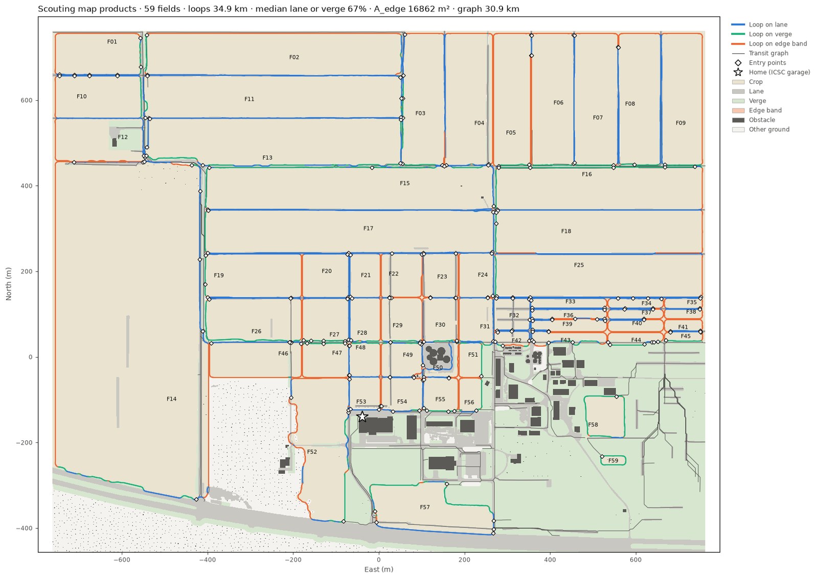
The loops over the ground classes. The loop colour is the class: blue on a lane, green on a verge, orange on the edge band. The transit graph is grey. The entries are diamonds. Home is a star.
Files#
The files are in Acres/Content/Simulation/ACRE/Scouting/. The other map data that the game reads at run time is in the
same parent folder. The packaged game includes this folder.
| File | Content |
|---|---|
scouting_map.json |
Schema acres-scouting-map-1. The build parameters, the hashes of the sources and home. The outline, loop, checkpoints, entries and statistics of each field. The transit graph and the statistics of the tile. |
ground_classes.u8 |
The ground class of each 0.5 m cell of the tile: 3048 × 3048 bytes, row 0 at the north edge (Git LFS). |
obstacles.json |
Schema acres-obstacles-1: the collision geometry of the level (buildings, bins, props, a parked car, 6,984 tree trunks). It is an input of the build. |
Positions are ENU metres about the tile centre (grid east and north; the enu_m of places.json). Each file of the
learning stack uses this frame. World metres are X = east, Y = −north. Unreal centimetres are X = 100 east, Y = −100
north. The raster cell of a point is row = (−north − origin) / step and column = (east − origin) / step. The origin is
−762.0015 m and the step is 0.500001 m (the layout of field_ids.u8).
acres_learn.tasks.scouting.map_products.ScoutingMap reads the files with numpy only. It works in the two conda
environments.
from acres_learn.tasks.scouting.map_products import ScoutingMap

m = ScoutingMap.load()
f = m.field("F39")
f.loop_xy, f.loop_class, f.loop_speed_limit      # 1 m apart, anticlockwise from the northernmost point
m.path("F39", entry=0, clockwise=True)           # the loop from an entry, in a driving direction
m.graph.shortest_path(m.home["graph_node"], f.entries[0]["node"])
m.ground_class(east, north)                      # class codes at points
Ground Classes#
| Code | Class | Content | Driving |
|---|---|---|---|
| 0 | Crop | The area of each field of fields.json that is not edge band, planted or fallow. |
Not permitted |
| 1 | Lane | surface_polygons.json classes grass_lane, asphalt, concrete, gravel, dirt. |
Permitted |
| 2 | Verge | Class grass outside the fields. |
Permitted |
| 3 | Edge band | Crop within the swept footprint of the vehicle along the edge-band stretches of the loops. | Permitted. The damage counts as unavoidable. |
| 4 | Obstacle | The collision geometry of obstacles.json. |
Not permitted |
| 5 | Other | Ground that is not field, lane or verge: the woodland floor south of US 52 and in the F52 woods, bare strips. | Not used by loops or transit |
The build paints the classes in this order: other ground, verge, crop, lane, obstacle, then the edge band over crop. A later class replaces an earlier class. A field painted over lawn is crop. Examples are the lawn fields F51, F55 and F56, and F58, which the surface layer still names grass.
A lane polygon inside a field is lane. Examples are the farm road through F52 and the plot alleys of F14. The first specification listed five classes. "Other" is the sixth class, because 57 ha of the tile are in none of the five.
The edge band is the crop within 1.0 m of the edge-band points of a loop. This distance is half the vehicle width plus 0.2 m. The band has two parts. The first part is the outer 2 m of the field where the loop is 1 m inside it.
The second part is the crop that a curvature-limited corner must cut. The band covers 18,000 m² of the tile. The body of the vehicle sweeps approximately the same area along the edge-band stretches (16,900 m²).
Scouting Loops#
The build makes each loop in six steps (build_map.py). Each step is a function.
1. Outline.
- \(B_f\) is the outer ring of the field, simplified with a 0.5 m tolerance.
- The outline has no holes. The loop goes around the outside.
- A closing bridges gaps and notches narrower than the turning circle (\(2R\) = 15 m). No loop of curvature ≤ 0.15 m⁻¹ can enter them.
- On 15 fields this removes more than a tenth of the ring. There the ring goes around an internal lane, or around a yard behind a lane gap. The ring of F04 runs 280 m up the two sides of an 8 m lane. The ring of F12 enters a lawn yard.
- The rings have 40.2 km in total. The scouting outlines have 35.9 km.
- The result is the scouting outline. It carries the offsets and the checkpoints.
2. Offsets.
- At each metre of the outline, the build finds an outward offset of 1.0-2.5 m at which the vehicle is on lane or verge.
- The centre line must be at least 1.0 m from crop or other ground. This is half of the 1.59 m width plus 0.2 m.
- The centre line must be 4 m from obstacles and 6 m inside the edge of the tile.
- The build takes the largest such offset. The exception is a smaller offset that keeps the vehicle further from crop (counted up to 2 m). An example is the 4.5 m lane between F11 and F13. The vehicle drives along its middle, not along its far side 1.0 m from the crop of the other field.
- Where no such offset exists, the offset is −1.0 m, which is the edge band. It is deeper where the edge of the tile is nearer.
- Where an obstacle is on the edge band, the build takes a wider offset on the lane (up to 6 m). The alternative is a deeper offset (up to 8 m). If the ground permits neither, it takes smaller clearances: 3 m, then 2 m, then half the vehicle width.
- The clearances give space to the driver. In a turn, the plan box of the vehicle sweeps up to 0.8 m outside the path of its rear axle. A learned policy moves further from the path. The policy of scout2 hit the shed adjacent to the lane of F58, where the loop passed 3.3 m from the wall. In the first build the clearance was 1.3 m. The body of the reference driver then touched the parked car adjacent to F54 and F55.
- The terrain ends at the edge of the tile. The reference point stays 6 m inside it, on a lane and on the edge band. The samples aim for 6.5 m, because the ramps of the corners bring the loop up to 0.5 m nearer.
- The policies of scout2 moved 3-4 m off their path (95th percentile 3.9 m outward). On each run of F18 their front wheels left the tile. The loop of F18 turned off a lane onto the edge band 4 m from the edge. The same occurred on 5 of 8 runs of F02, where the loop was on the lane along the north edge, 3.5 m from it.
- Thus F01 and F02 now use their own edge band adjacent to that lane. Their lane is 1-5 m from the north edge. Their unavoidable crop was 194 and 246 m² and is now 475 and 981 m². F02 is no longer 90 % lane-bound.
3. Profile. The build opens the offsets along the outline with a parabolic structuring function of curvature \(1/R\), \(R\) = 7.5 m. The profile is never more than the feasible offset. Each change between the lane and the edge band becomes a ramp approximately 7 m long.
4. Region. The build draws the area inside the offset line on a 0.25 m raster. It closes and opens the area with a disc of radius \(R\) (exact Euclidean morphology with distance transforms). Thus its boundary bends no tighter than \(1/R\) = 0.133 m⁻¹ in each direction. This is below the limit and leaves a margin for the discretisation.
5. Trace and repair.
- The build traces the boundary and smooths it along its length (Gaussian, 1 m). It samples the boundary again at 1 m intervals and rounds it to the millimetre.
- The opening can cut a corner across a tree in the crop. The boundary can then pass closer than 3 m to an obstacle. There the build adds a disc of radius \(R\) around the far side of the obstacle, or cuts one from its near side. Then it smooths and traces the region again. It does this at most five times. One pass can repair more than one place.
- Two fields need this repair. F49 has a parked car in the lane (2.98 m). F52 has trees in a thin lobe of the field (2.74 m after eight repairs).
- A hairpin is a place where a loop turns by 150° or more within 35 m. Most hairpins are on the edge band, at the ends of the 24 m strips F33-F45. These strips border each other and have no lane between them.
- At a hairpin, the two corners of radius \(R\) become one turn of up to 11 m radius. The build opens the region there with a disc of that radius, no wider than the strip permits. It keeps the result if the loop still covers the same number of checkpoints.
- The reason is the lateral acceleration. Two corners of 7.5 m need 4.0 m/s² at 5.5 m/s. One turn of 11 m needs 2.7 m/s². Through crop, the vehicle has only the path to follow. Each run of the policies of scout2 drove on along the lane of F33.
- Nine fields have a rounded hairpin: F33, F34, F36, F37, F39, F40, F43, F44, F52.
- Some fields are too narrow for this method. F50 is an L of lawn strips approximately 10 m wide, between the bin yard and the lawn fields F51, F55 and F56. The opening removes its region, and the loop misses its checkpoints.
- When a loop covers less than 95 % of its checkpoints, the build makes it again from a region that is 2 R wide. This region is the field without its 1 m edge band, plus lane and verge near it. The region includes lane and verge within 16 m minus the local thickness of the strip. The local thickness is the diameter of the largest disc inside the strip, the largest within 3 m. The build closes, opens and closes the region. The opening of a rough region can leave a narrow point where two of its discs meet.
- The loop then goes up the open side of the strip, some metres out on the yard, and back along its edge band.
6. Classes and speed limits. A point is lane or verge when the whole footprint of the vehicle is off crop and off other ground. It is lane when the ground below its centre is lane. Each other point is edge band.
The speed limit is 5 m/s on lane and verge and 3 m/s on the edge band. It is lower in corners, where the lateral acceleration must be at most 1.5 m/s²: \(v \le \sqrt{1.5 / \lvert\kappa\rvert}\). This is 3.2 m/s at the tightest curvature, 0.15 m⁻¹.
The curvature comes from the circle through the points 2 m before and 2 m after each point. Thus noise below 1 m does not count. Positive curvature is to the left.
The unavoidable crop area of a loop is its edge-band length times the width that the Polaris crushes: \(A^\text{edge}_f = 1.59\,\text{m} \times L^\text{edge}_f\). The body sweeps crop that is taller than 0.33 m. Each crop of the map is taller (corn 2.4 m, soybean 0.5 m, potato 0.55 m). Thus the crushed width is the full 1.59 m of the vehicle, not the 0.56 m of its tyre tracks. The game and ACRES Core give the same measurement.
The file stores each loop anticlockwise from its northernmost point. The values for each point are east_m, north_m,
class, speed_limit_mps, curvature_per_m and offset_m. offset_m is the signed distance to \(B_f\), positive
outside. The clockwise loop is the same points in reverse order, with the opposite sign of the curvature.
Checkpoints#
The checkpoints have an even spacing along the scouting outline: 10 m or a little less. The first checkpoint is at the point nearest the start of the loop. The 59 fields have 3,614 checkpoints. A checkpoint is covered when the reference point of the vehicle passes within 8 m of it. A field is scouted at 95 % coverage with the vehicle again at its entry.
A drive along the loop covers at least 95.8 % of the checkpoints of each field:
| Coverage | Fields |
|---|---|
| 100 % | 46 fields |
| 95.8 % | F35 and F45 (small plots at the east edge of the tile; their loops now keep 6 m from the edge) |
| 96.2 % | F41 (the same cause) |
| 97.1 % | F50 (the narrow strip above) |
| 97.4 % | F58 |
| 98-99 % | Eight fields with tight corners that the loop cannot follow |
Entry Points and the Transit Graph#
The transit graph has two sources. The first source is the lane centre lines of the surveyed lane layer
(Calibration/Map/Layers/lanes.geojson). The second source is the roads of site.json that the NPC road graph of the
game uses (FAcresRoadGraph). These are the roads narrower than 20 m, thus not US 52. The graph uses a road only where
no surveyed centre line is within 3 m.
The build keeps each line where it is on lane or verge. The line must also be at least 2.0 m from obstacles and 18 m from the centre line of US 52. It resamples the line at 5 m intervals. It merges points within 4.5 m into shared nodes, as the NPC graph does.
That network has 96 pieces. Lanes end at yards, lots and lawns that have no centre line. The build joins the pieces with least-cost routes on a 1 m grid. The cost is 1 per metre on lane and 1.3 per metre on verge. For pieces that are still not reachable, the route can use the edge band at 20 per metre. The specification permits a transit on the edge band only where no other connection exists.
This occurs only among the plot fields F33-F45. Their shared edges isolate their lane stubs. There are 13 such connectors (643 m). The build removes pieces that no route reaches (alleys closed in by crop). H is the ICSC garage spawn (cell u 474.6, v 592.2, heading north). It joins the graph by a 12 m route.
The entries \(K_f\) of a field are junctions and ends of the graph. They are within 6 m of the lane and verge points of the loop. The first build used 5 m. A move of a loop by some centimetres then removed the south-west junction of F05.
A field has one entry for each 10 m of loop at most, and at most 6. The build keeps the most spread-out entries along the loop. Each entry is a node on the loop, linked to its junction. F59 is a lawn plot with no lane near it. It gets its entry by a routed connector.
Most entries are in a corner of their loop, where lanes cross. A test put the entries on the straight adjacent to the
corner. The link of such an entry is along the loop. A vehicle that has come around the loop cannot leave by such a link
without a turn. In the test, 53 of the 59 single-field reference plans reversed at some point, against 39 now. The loop
stage of the flat-policy curriculum can start its episodes on that straight (loop_start: straight,
Training).
The stored graph keeps nodes only at junctions, ends, entries and H: 505 nodes, 516 undirected edges, 30.9 km. Each edge
has its polyline and its length. It has the ground class that covers most of its length (lane, road, connector,
edge_band_connector, entry) and its length for each kind. edge_band_m is the part that a planner must price as
edge band.
Measured Statistics#
| Measure | Value |
|---|---|
| Loops | 59 closed, 34.9 km in all, 145-2202 m (median 387 m) |
| Largest curvature | 0.148 m⁻¹ (limit 0.15) |
| Share of the loop on lane or verge | median 67 %; ≥ 90 % on 11 fields, 70-90 % on 14, 50-70 % on 17, < 50 % on 17 |
| Least lane-bound | F05 17 %, F40 27 %, F41 33 %, F46 38 %, F38 39 % |
| Unavoidable crop \(A^\text{edge}\) | 16,862 m² in all (15,871 before: F01 and F02 off their lane), median 183 m² per field; most on F14 (2,110 m²) |
| Checkpoint coverage by the loop | ≥ 95.8 % on every field |
| Obstacle clearance | ≥ 3.66 m on every field but two. F52: 2.74 m (trees in a thin lobe). F49: 1.97 m (a clearance of 3 m from the car at its corner costs a checkpoint). The vehicle half-width is 0.8 m |
| Tile edge | the reference point ≥ 6.0 m inside the tile on every loop; the wheels ≥ 4.8 m |
| Hairpins rounded | 9 fields (F33, F34, F36, F37, F39, F40, F43, F44, F52) |
| Entry points | 1-6 per field, 229 in all |
| Transit graph | 30.9 km: lane 16.6, road 4.9, connector 8.2, edge band 0.6, entry links 0.6 |
The specification has its own measure: the 2.5 m offset of \(B_f\), with the centre line on lane or verge. By that measure the median is 73 %, 11 fields are at least 90 % and 9 are under 50 %. The specification quotes 76 %, 13 and 10. The share of the loops is different for two reasons. The loops keep the whole vehicle off crop, not only its centre line. A corner cut through the crop of an adjacent field counts as edge band.
Nineteen fields reach the edge of the tile. They are the north row F01-F09, F10, F12 and F14 in the west, and F16-F45 in the east. The simulator models nothing outside the tile. Thus their loops stay 6 m inside it, on the edge band or on a lane along the edge. The samples aim for 6.5 m, and the ramp of a corner comes up to 0.5 m nearer.
The corner cuts and the edge band along the edge of the tile are up to 8.4 m inside a field (F09). The loop of F52 cuts 4.5 m inside its outline where it crosses the farm road. That stretch is edge band. Thus an environment must test "more than 6 m inside crop" against the edge-band raster, not against the distance to \(B_f\).
The table gives these values for each field:
- The area (ha).
- The length of the loop (m) and its shares of lane, verge and edge band (%).
- The unavoidable crop \(A^\text{edge}\) (m²).
- The number of entries.
- The share of the checkpoints that the loop covers (%).
| Field | Area | Loop | Lane | Verge | Edge Band | \(A^\text{edge}\) | Entries | Coverage |
|---|---|---|---|---|---|---|---|---|
| F01 | 1.95 | 577 | 37 | 12 | 52 | 475 | 6 | 98 |
| F02 | 5.99 | 1375 | 48 | 7 | 45 | 981 | 2 | 100 |
| F03 | 2.89 | 797 | 59 | 27 | 14 | 178 | 6 | 99 |
| F04 | 3.19 | 828 | 39 | 1 | 60 | 787 | 2 | 99 |
| F05 | 2.74 | 781 | 8 | 9 | 83 | 1036 | 4 | 100 |
| F06 | 3.04 | 803 | 44 | 12 | 44 | 566 | 4 | 100 |
| F07 | 3.05 | 806 | 71 | 12 | 17 | 218 | 4 | 100 |
| F08 | 2.91 | 796 | 72 | 11 | 16 | 207 | 2 | 99 |
| F09 | 3.09 | 792 | 38 | 11 | 50 | 634 | 1 | 99 |
| F10 | 1.94 | 587 | 67 | 16 | 17 | 161 | 4 | 100 |
| F11 | 5.64 | 1395 | 96 | 3 | 0 | 8 | 6 | 100 |
| F12 | 1.53 | 611 | 65 | 0 | 35 | 335 | 4 | 98 |
| F13 | 6.00 | 1394 | 71 | 29 | 1 | 16 | 6 | 100 |
| F14 | 25.98 | 2202 | 30 | 10 | 60 | 2110 | 6 | 100 |
| F15 | 6.26 | 1533 | 56 | 43 | 1 | 14 | 6 | 100 |
| F16 | 4.58 | 1153 | 43 | 48 | 9 | 165 | 6 | 100 |
| F17 | 6.33 | 1532 | 93 | 6 | 1 | 27 | 6 | 100 |
| F18 | 4.73 | 1158 | 82 | 8 | 9 | 168 | 3 | 100 |
| F19 | 2.17 | 640 | 68 | 15 | 17 | 172 | 4 | 100 |
| F20 | 1.05 | 410 | 75 | 0 | 25 | 166 | 2 | 100 |
| F21 | 0.68 | 336 | 69 | 0 | 31 | 164 | 2 | 100 |
| F22 | 0.96 | 385 | 41 | 0 | 59 | 361 | 3 | 100 |
| F23 | 0.85 | 360 | 40 | 0 | 60 | 342 | 4 | 100 |
| F24 | 0.80 | 357 | 67 | 0 | 33 | 189 | 3 | 100 |
| F25 | 4.65 | 1162 | 67 | 8 | 25 | 466 | 4 | 99 |
| F26 | 2.00 | 629 | 37 | 47 | 16 | 162 | 4 | 100 |
| F27 | 1.01 | 405 | 49 | 25 | 25 | 164 | 6 | 100 |
| F28 | 0.67 | 334 | 55 | 13 | 32 | 170 | 2 | 100 |
| F29 | 0.91 | 384 | 35 | 16 | 50 | 304 | 4 | 100 |
| F30 | 0.72 | 363 | 28 | 12 | 61 | 350 | 4 | 100 |
| F31 | 0.78 | 362 | 62 | 6 | 31 | 181 | 2 | 100 |
| F32 | 0.55 | 310 | 95 | 0 | 5 | 22 | 6 | 100 |
| F33 | 0.33 | 388 | 93 | 0 | 7 | 41 | 3 | 100 |
| F34 | 0.25 | 289 | 79 | 0 | 21 | 96 | 6 | 100 |
| F35 | 0.19 | 212 | 78 | 0 | 22 | 75 | 2 | 96 |
| F36 | 0.34 | 387 | 66 | 0 | 34 | 208 | 6 | 100 |
| F37 | 0.26 | 289 | 65 | 0 | 35 | 159 | 3 | 100 |
| F38 | 0.21 | 210 | 39 | 0 | 61 | 205 | 1 | 100 |
| F39 | 0.47 | 391 | 41 | 0 | 59 | 368 | 6 | 100 |
| F40 | 0.36 | 298 | 27 | 0 | 73 | 345 | 1 | 100 |
| F41 | 0.25 | 220 | 33 | 0 | 67 | 233 | 2 | 96 |
| F42 | 0.24 | 218 | 56 | 11 | 33 | 113 | 5 | 100 |
| F43 | 0.38 | 408 | 31 | 20 | 49 | 315 | 6 | 100 |
| F44 | 0.30 | 296 | 11 | 31 | 58 | 272 | 6 | 100 |
| F45 | 0.17 | 207 | 36 | 41 | 24 | 78 | 4 | 96 |
| F46 | 1.70 | 581 | 37 | 1 | 62 | 577 | 4 | 100 |
| F47 | 0.85 | 365 | 19 | 28 | 53 | 305 | 5 | 100 |
| F48 | 0.55 | 292 | 52 | 17 | 31 | 145 | 2 | 100 |
| F49 | 0.66 | 334 | 53 | 13 | 34 | 183 | 6 | 100 |
| F50 | 0.14 | 335 | 62 | 3 | 34 | 183 | 3 | 97 |
| F51 | 0.41 | 256 | 12 | 37 | 52 | 210 | 1 | 100 |
| F52 | 3.57 | 949 | 31 | 21 | 48 | 726 | 4 | 100 |
| F53 | 0.49 | 286 | 72 | 0 | 28 | 129 | 4 | 100 |
| F54 | 0.66 | 335 | 65 | 6 | 29 | 154 | 6 | 100 |
| F55 | 0.60 | 302 | 40 | 26 | 34 | 162 | 6 | 100 |
| F56 | 0.39 | 247 | 14 | 35 | 51 | 200 | 1 | 100 |
| F57 | 2.31 | 766 | 51 | 44 | 5 | 65 | 6 | 100 |
| F58 | 0.76 | 360 | 8 | 90 | 2 | 14 | 1 | 97 |
| F59 | 0.08 | 145 | 0 | 99 | 1 | 2 | 1 | 100 |
Where the Products Depart from the Specification#
- Offsets between 1.0 and 2.5 m. The specification puts the loop 2.5 m outside \(B_f\) or 1.0 m inside. Some lanes are narrower than 2.5 m plus the clearance. There the loop stays on the lane at a smaller offset (down to 1.0 m). It does not crush crop.
- The whole vehicle, not only its centre line. A point is lane or verge only when the whole footprint of the vehicle is off crop. Thus a drive along the loop never crushes crop that the reward counts outside the edge band.
- Bridged outlines. The loops and the checkpoints use \(B_f\) with gaps narrower than 15 m bridged. The strips of field inside such a gap have no checkpoints. An example is a lane that the field goes around.
- Margins for a learned driver. The loop of the specification is the path of a careful driver. The products leave space for a driver that moves 3-4 m off the path, as the stage-1 policy of scout2 did. The margin from the edge of the tile is 6 m. The margin from obstacles is 4 m where the ground permits it, else 3 m, then 2 m. The loop of a narrow lane is along its middle. A hairpin through crop is one turn of up to 11 m. The first build kept 3 m from the edge of the tile plus half the vehicle width, and 2.5 m from obstacles. It took the largest offset on a lane and ignored the crop on the far side.
- A sixth class. Ground outside each field, lane and verge is "other".
- Crushed width 1.59 m. \(A^\text{edge}_f\) counts the sweep of the body (1.59 m for each metre). The specification stated the 0.56 m of the tyre tracks. The body of the Polaris crushes crop taller than 0.33 m, and each crop of the map is taller. The crop reward of the task uses \(A_\text{ref}\) = 1.59 m × 0.4 m = 0.636 m² to agree. This keeps its scales for each step (−5 fully in crop, −0.2 on the edge band).
- Routed connectors. Routes on lane and verge join the lanes and roads of the transit graph over yards, lots and lawns. The specification names only centre lines. Centre lines only leave the network in 96 pieces.
Rebuilding#
Use the torchenv conda environment. Start in Learning/.
-
Extract the obstacles. Do this step only when the structures or the trees of the level change.
-
Build the products. This takes approximately 25 s and writes
scouting_map.jsonandground_classes.u8. -
Draw the figures:
overview.pngandfield_Fxx.pngfor each field. -
Run the tests.
The obstacle extraction reads two dumps of the level that are not in the repository. They are
Acres/Saved/structures_level.json from the level tools and the T20 tree dump below $POLARIS_EPISODES. The build
reads only committed files and is deterministic. The build parameters are the map section of
Learning/acres_learn/configs/scouting_v1.json. The map records the hash of this section with the hashes of its
sources.
Learning/tests/test_scouting_map.py checks the committed products:
- Each field has a closed anticlockwise loop with points 1 m apart.
- The curvature is ≤ 0.15 m⁻¹ (calculated again from the points).
- The classes and the speed limits follow the rules above.
- No loop point is on crop outside the edge band or within 1.0 m of an obstacle.
- The checkpoints are at most 10 m apart, and the loop covers at least 95 % of them.
- Each field has 1-6 entries.
- The transit graph joins all entries to H and stays off obstacles. It crosses crop only at junction corners (44 m of 30.9 km).
The test also checks the margins:
- Each loop point is 6 m or more from the edge of the tile.
- The wheels of a vehicle on a loop, in each direction, are at least 4.5 m inside the tile.
- The termination test uses a wheel off the tile, not the body.
- Each loop is 3 m from obstacles. The exceptions are places where the ground permits no more. There a sideways move of the loop to 3 m puts the vehicle on crop, other ground or an obstacle. A second exception is a place where 3 m costs a checkpoint (F49).
- The loop of F58 is 4 m from the shed.
- The loop on the 4.5 m lane between F11 and F13 is along the middle of the lane.
- The hairpin of F33 is rounded.
Limitations#
- The collision geometry of the level is an approximation. Buildings are their placed outlines or footprints. Bins and trunks are cylinders. Props and the parked car are their bounding boxes. The east elevator leg is a 6 m square, because its bounds include the spouts. The obstacle layer is only as current as its source, the level dumps.
- Graph corners. The nodes of the transit graph are 2-5 m apart and merge within 4.5 m. Thus a chord can cut a field corner by up to 4 m (44 m of crop over the whole graph).
- The lane network is as surveyed. Lanes that the survey did not record change the loops and the graph. Lanes that the survey shows but that are no longer mown change them too. Yards inside field polygons have the same effect. The west bin yard of F50 (4,800 m² of gravel with six bins) is no longer a part of the field: The ACRE Scene.